Fructivore Investments

Have you, like me, ever wondered how you might derive the zero curve from the par yield curve but don’t know where to start? If so, I have good news for you.

The yield curve, or more formally, the term structure of interest rates, is a vital tool for any fixed income analyst, and also of non-trivial interest for anyone who has anything to do with borrowing money. But how to construct the yield curve? What yield to use?

A good place to start in the United States is the yield on Treasury instruments, because Treasuries avoid the issues of credit risk, liquidity risk, and callability that plague other bonds, and those other risks can be assessed later. But even Treasuries offer their choice of yield curves. The first yield formula they teach you at yield curve formula school is the yield to maturity, but that formula assumes that all interim payments are reinvested at the same rate, which is a highly questionable assumption unless the yield curve itself is flat, which it never is. So one would expect the yield to maturity to have fallen by the wayside decades ago.

There is, however, a measure of yield that is completely agnostic as to reinvestment assumptions, and that is the zero curve. The zero curve treats every coupon from the bond as a separate maturity with no interim coupons to reinvest, so it is a much better approximation of the one true yield. One could, of course, call our friendly neighborhood investment banker or fire up the old Bloomberg for quotes on zeroes of various maturities, but there are data quality issues and not all of us have an investment banker on call.

Fortunately, the US Treasury, posts a daily yield curve we can use. Unfortunately, the Treasury publishes the par yield for any coupon bonds, not the zero curve. The par yield is a measure of what coupon rate would cause a bond with the stated maturity to trade at par, which Treasury assures us that they calculates using the finest and rarest of algorithms. The trouble is that as far as I can tell, the par yield can only be constructed from the zero curve, so the US Treasury has just added a step to our process that must be patiently undone. Fortunately analysts are accustomed to doing this anyway when dealing with accountants when examining a company’s financial reports.

Furthering our inconvenience, the Treasury doesn’t publish every rate, or even every yearly rate. It is kind enough to give us the six month and one year par rates, and it is simple algebra to compute the zero rates on a one year bond from these inputs. (I say simple algebra, but the one year rate must be solved numerically, which Excel is perfectly capable of). The method is essentially the same method as bootstrapping a forward rate curve.

However, the next par rate published by the Treasury is the 2 year rate, which is a problem because Treasuries pay semiannually, which means that even if we have the 6 month and 1 year rates, there are two interest rates to solve for here with only one equation, meaning that we have an infinite number of solutions.

Let us suppose, however, that the 18 month rate and the 2 year rate are mathematically related to each other in some manner, such as linearly. In other words, the 1 year rate + r equals the 18 month rate, and the 18 month rate plus r equals the 2 year rate. Brilliant, you think; we have just added a third variable to our problem. But in fact we have defined the 18 month rate and 2 year rate in terms of the one year rate and a single variable, making this an equation that we, and by “we” I mean Excel, can easily solve. And we may continue in this vein with the other stated Treasury par yield dates to fill in the entire yield curve for 30 years.

This will give us a nice chunky polygon which will somewhat resemble the par curve but generally with a slightly exaggerated slope. This is the one prepared using the published Treasury par yield curve of January 2, 2024.

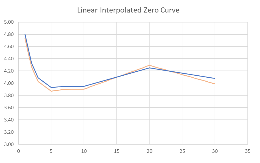
The blue is the par yield curve; the orange is the calculated zero curve. It is usable, but I think there is room for improvement. It makes no sense to me that a yield curve should be discontinuous at each Treasury-published rate, as in my view a yield curve develops organically from the views of market participants and even if some participants are bound to bonds of a particular maturity, other participants are not, and even if the holder of a 2 year bond may not care about the yields on a 25 year bond, they should care about the yields on a 3 year bond, so some smoothing is in order.

So, what can we do? We can enforce continuity by assuming that the outgoing slope of one yield curve section will equal the incoming slope of the next section, and within the section use an approximation other than linear. The Treasury itself uses cubic hermite splines, but after extensive fiddling in Excel I’ve found that at least a sensible-looking graph can be created by using two methods, one by using a natural log function instead of linear, and also allowing the slope of the graph to shift from the incoming slope in each section to the slope implied by the next section (or zero, in the case of the 20-30 year), because I found that a pure backward-looking method was producing distortions because, as stated above, the 2 year and the 3 year interest rates, for example, should have some influence on each other because at least some market participants are capable of choosing between the two when constructing their portfolios.

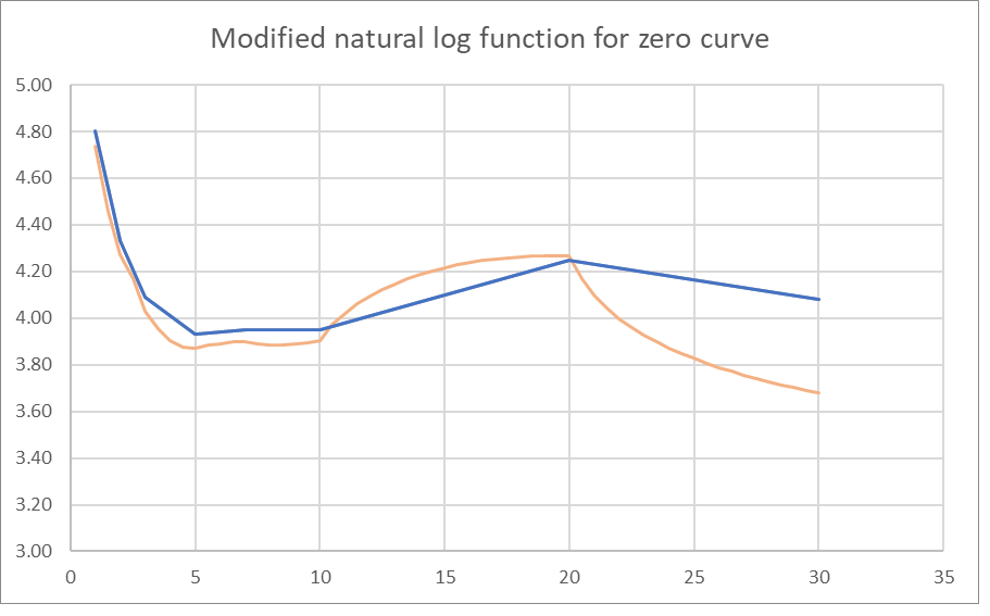
Unfortunately, the Treasury does not publish rates between the 10, 20, and 30 year rates, and the unusual shape of the yield curve of January 2, 2024, which inverts, uninverts, and then reinverts, makes a wonky shape of the 20-30 year section no matter what reasonable modifications are attempted. I assume the natural log term is useful because, based on my observations, the yield curve tends towards flatness as opposed to more extreme slopes as yields extend into the future, and anyone who claims a genuine insight as to whether the difference between the 28 and 29 year rate should be larger than the 27-28 year rate spread had better have a very good reason for making such a claim.

So, now that we have this cool curve, what are the applications? The benefit of casting the yield curve in sections of functions with defined coefficients that we have solved for is that we can calculate the interpolated rates at any future date, not simply at six month intervals, which will be helpful for the 363 days a year which are not the coupon days. And with these zero curves on any particular date we can apply them to any corporate, as opposed to Treasury bond, and neatly and accurately compute the zero volatility spread offered by that particular bond, in order to search for anomalies that may represent attractive investment opportunities, or, more ambitiously to work out a term structure of zero volatility spreads across several bonds, which may be of interest when constructing a fixed income portfolio, or even to evaluate multiple bonds of the same issuer to see if the market is anticipating some change in the financial situation of one issuer over time.

Also, getting back to yield to maturity, we can also calculate any implied forward rate we like. I said the flaw with the yield to maturity is that we assume that all intermediate cash flows must be reinvested at the same rate. But with this method we can instead assume that intermediate cash flows can be reinvested at the forward rate implied by the yield curve, and discount that future value back to present value, thus possibly identifying attractive opportunities among Treasury instruments or among corporate instruments with the same credit spreads, or even work out a term structure of the gaps between yield to maturity and forward curve implied spreads. I do not recall seeing anyone using this method, but it is a way of sieving out anomalies, and for analysts, anomalies are in theory worth investigating.

Filed under:
Investing by grocca